In the previous post, I wrote about the exponential and its definition as the function proportional to its first derivative, namely:

$\begin{aligned} &\frac{dy}{dt}+\lambda y(t)=0~.&(1) \end{aligned}$

There are many functions of mathematics that derive from differential equations like this one. Take the following example where the funtion of a single space variable, $y(x)$, is not just proportional to its first derivative, but rather satisfies

$\begin{aligned} &\frac{dy}{dx}+\frac{x}{\sigma^2}y(x)=0~,&(2) \end{aligned}$

where $\sigma$ is a constant real number. In order to solve the above we can use the technique of separation of variables (pardon the lack of mathematical rigour):

$\begin{aligned} \frac{dy}{dx}&=-\frac{x}{\sigma^2}y(x)\\[1em] \leftrightarrow \int\frac{dy}{y}&=-\int\frac{x}{\sigma^2}dx\\[1em] \leftrightarrow \log(y)&=-\frac{1}{2}\frac{x^2}{\sigma^2}+B\\[1em] \leftrightarrow y(x)&=Ae^{-\frac{1}{2}\frac{x^2}{\sigma^2}}~,&(3) \end{aligned}$

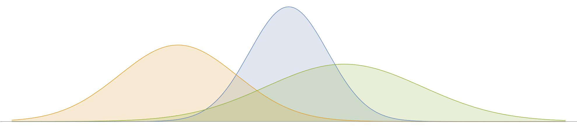
where $\log(x)$ is the natural logarithm (the inverse of the exponential function, $e^x$) and $A$ and $B\equiv \log{A}$ are constants. This function is the gaussian function centred at the origin and has many applications in many areas of mathematics including probability theory, statistics, information theory, quantum mechanics, etc… Equation (2) is a perfectly valid – although not very common – definition of this function and has the advantage of explicitly showing some of the function’s properties. For example, it is invariant under the transformation that takes $x$ to $-x$, contrary to Eq.(1) when $t$ goes to $-t$.

By taking the derivative on both sides of Eq.(1), we obtain the following second order differential equation :

$\begin{aligned} &\frac{d^2y}{dx^2}+\frac{\sigma^2-x^2}{\sigma^4}y=0~.&(4) \end{aligned}$

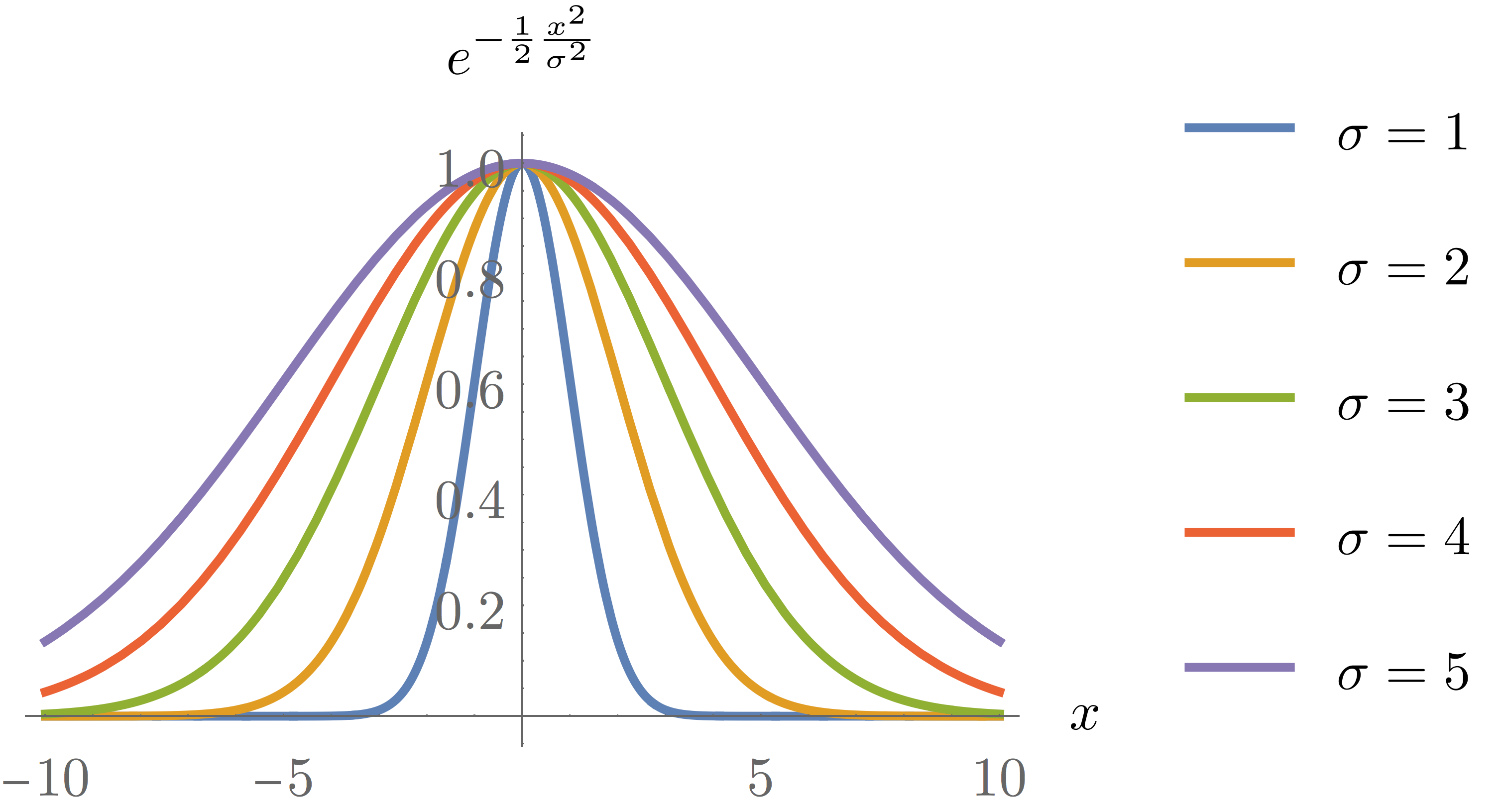
Since the sign of $y$ is constant for all values of $x$, this means that $\frac{d^2y}{dx^2}$ changes sign at $x=\pm\sigma$ corresponding to the location of inflection points in the original function. By inserting these values back into Eq.(3), we find that these correspond to $y(\pm\sigma)=\frac{A}{\sqrt{e}}\approx0.607 A$. You can see the plot of the function for different values of $\sigma$ on the figure below.

Because of its shape, the gaussian function is sometimes referred to as the bell curve. From Eq.(\ref{eq:dydx}), we see that its first derivative is simply (assuming $A=1$)

$\frac{dy}{dx}=\frac{x}{\sigma^2}e^{-\frac{1}{2}\frac{x^2}{\sigma^2}}~.$

Its first integral, however, cannot be evaluated in terms of simple functions. There is however a notable exception when the integral covers the entire real line:

$\begin{aligned} &I\equiv\int_{-\infty}^{\infty}e^{-\frac{1}{2}\frac{x^2}{\sigma^2}}dx=?&(5) \end{aligned}$

The trick is to start by taking the square of the above and then change to the polar set of coordinates

$\begin{aligned} I^2&=\int_{-\infty}^{\infty}e^{-\frac{1}{2}\frac{x^2}{\sigma^2}}dx\int_{-\infty}^{\infty}e^{-\frac{1}{2}\frac{y^2}{\sigma^2}}dy\\[1em] &=\int_{-\infty}^{\infty}\int_{-\infty}^{\infty}e^{-\frac{1}{2}\frac{x^2+y^2}{\sigma^2}}dxdy\\[1em] &=\int_{0}^{2\pi}d\theta\int_{0}^{\infty}r e^{-\frac{1}{2}\frac{r^2}{\sigma^2}}dr~. \end{aligned}$

The integrand on the right is equivalent to the right-hand-side of Eq.(2) where $x\rightarrow r$. By substituting the left-hand-side, we arrive at

$\begin{aligned} I^2&=2\pi\sigma^2\int_{0}^{\infty}\frac{d}{dr}e^{-\frac{1}{2}\frac{r^2}{\sigma^2}}dr\\[1em] &=2\pi\sigma^2 \left\{e^{-\frac{1}{2}\frac{r^2}{\sigma^2}}\right\}_{0}^\infty\\[1em] \leftrightarrow I&=\sqrt{2\pi}~\sigma~. \end{aligned}$

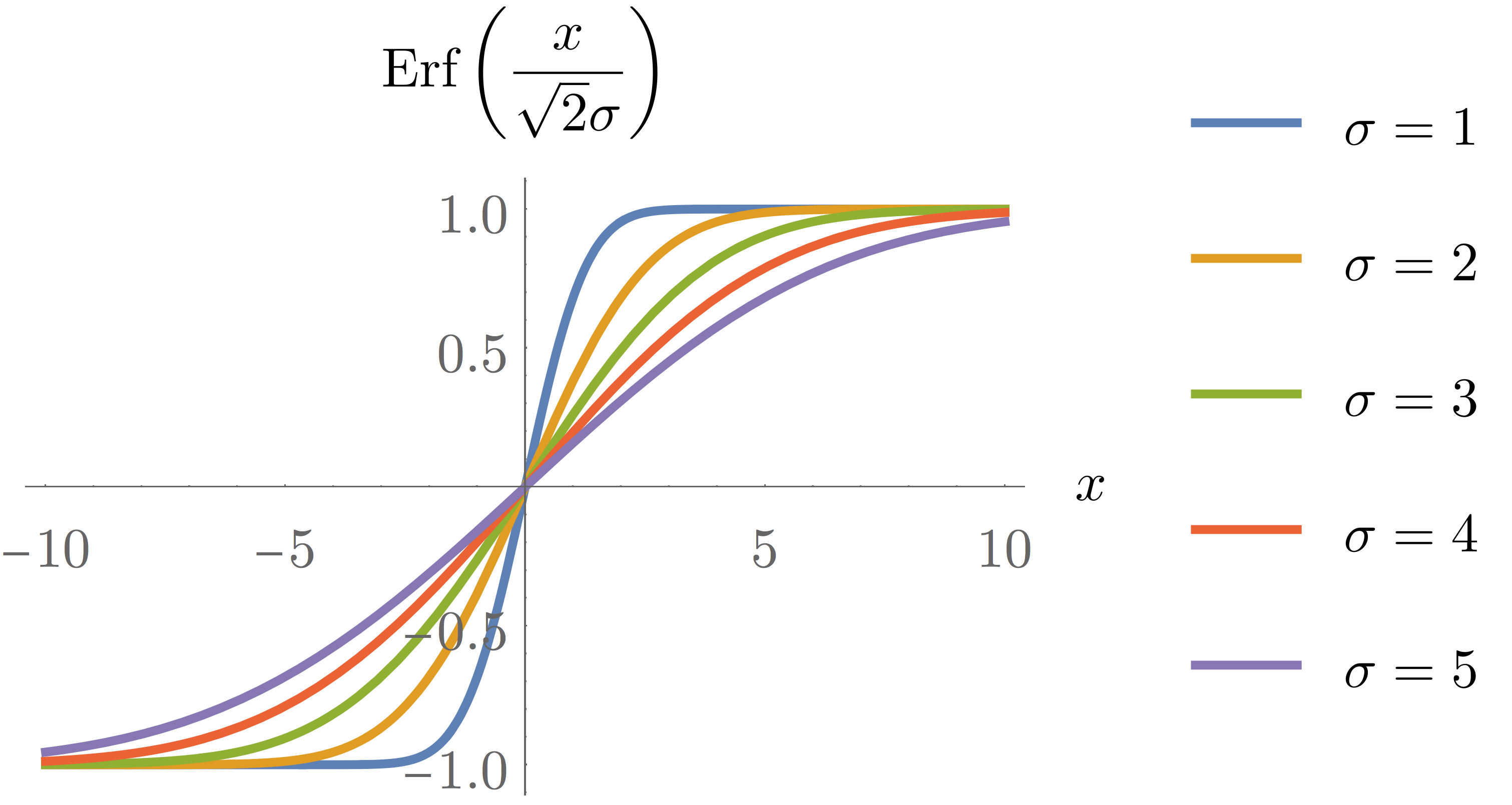
The Error function is a special case of Eq.(5) defined as

$\begin{aligned} \text{Erf}(x)&=\frac{2}{\sqrt{\pi}}\int_0^xe^{-u^2}du\\[1em] \text{Erf}\left(\frac{x}{\sqrt{2}\sigma}\right)&=\frac{2}{\sqrt{2\pi}\sigma}\int_0^xe^{-\frac{1}{2}\frac{u^2}{\sigma^2}}du&(6) \end{aligned}$

The figure below shows the plot of Eq. (6) for different values of $\sigma$.

From Eq. (4) and the definition of the error function, one can compute the following weighted gaussian integral:

$\begin{aligned} \int_0^x \frac{u^2}{\sigma^2}e^{-\frac{1}{2}\frac{u^2}{\sigma^2}}du&=\int_0^x e^{-\frac{1}{2}\frac{u^2}{\sigma^2}}du+\sigma^2\int_0^x \frac{d^2}{du^2}\left(e^{-\frac{1}{2}\frac{u^2}{\sigma^2}}\right)du\\[1em] &=\int_0^x e^{-\frac{1}{2}\frac{u^2}{\sigma^2}}du+\sigma^2\left\{\frac{d}{du}\left(e^{-\frac{1}{2}\frac{u^2}{\sigma^2}}\right)\right\}_0^x\\[1em] &=\sqrt{\frac{\pi}{2}}\sigma~\text{Erf}\left(\frac{x}{\sqrt{2}\sigma}\right)-e^{-\frac{1}{2}\frac{x^2}{\sigma^2}}x~. \end{aligned}$